Insights into Transformer-Based GNSS Correction Network

Improving real-time smartphone positioning accuracy with deep learning—particularly a Transformer-based GNSS Positioning Correction Network—requires careful decisions about both data preprocessing and model design. This article records the main ideas and results from that project.

1. Weighted Least Squares recap

Weighted Least Squares (WLS) is a common baseline for GNSS positioning. It solves an overdetermined system formed by pseudorange equations from multiple satellites.

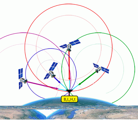
The basic GNSS pseudorange equation is

$$P_i = \sqrt{(x_{\text{sat},i} - x_{\text{rec}})^2 + (y_{\text{sat},i} - y_{\text{rec}})^2 + (z_{\text{sat},i} - z_{\text{rec}})^2} + c \cdot \Delta t_{\text{rec}} + \varepsilon_i.$$

Here:

• $P_i$ is the pseudorange from satellite $i$;
• $(x_{\text{sat},i}, y_{\text{sat},i}, z_{\text{sat},i})$ are the satellite’s ECEF coordinates;
• $(x_{\text{rec}}, y_{\text{rec}}, z_{\text{rec}})$ is the unknown receiver position;
• $c \cdot \Delta t_{\text{rec}}$ is the receiver clock bias term;
• $\varepsilon_i$ is measurement noise.

There are usually more satellites than the four unknowns $\{x_{\text{rec}}, y_{\text{rec}}, z_{\text{rec}}, \Delta t_{\text{rec}}\}$, so WLS linearizes the system and iteratively solves

$$\Delta \mathbf{x} = (\mathbf{H}^T \mathbf{W} \mathbf{H})^{-1} \mathbf{H}^T \mathbf{W}\bigl(\mathbf{z} - \mathbf{r}(\mathbf{x}_0)\bigr).$$

Where:

• $\mathbf{z}$ contains the measured pseudoranges $P_i$;
• $\mathbf{r}(\mathbf{x}_0)$ is the modeled pseudorange from the current estimate;
• $\mathbf{H}$ is the Jacobian matrix;
• $\mathbf{W}$ is a diagonal weight matrix;
• $\Delta \mathbf{x}$ updates the receiver position and clock bias.

After a few iterations, WLS converges to $\hat{\mathbf{x}}$. This solution becomes the baseline that the deep-learning model attempts to refine.

2. Motivation for deep learning in GNSS positioning

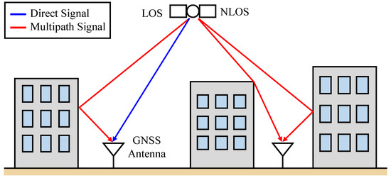
Urban environments can severely degrade GNSS signals through multipath and Non-Line-of-Sight (NLOS) effects. Traditional WLS-based methods are not always robust enough under these conditions. Deep learning can capture nonlinear relationships and subtle patterns in the observations, potentially producing a more accurate correction.

Why not directly regress coordinates?

Two problems make direct regression difficult:

1. Large numeric ranges. Raw pseudorange values can be on the order of $10^5$ meters, which risks unstable gradients.
2. Permutation invariance. The order of satellite observations in an epoch should not affect the result, but a normal sequence model still sees an order.

The preprocessing and output formulation therefore need to be designed before the measurements enter the Transformer.

3. Data preprocessing

3.1 Rethinking data filtering

Rather than discarding noisy measurements—such as low-elevation signals—we kept them all. Noise can encode environmental clues, including multipath behavior. The attention mechanism can learn to downweight unreliable signals instead of relying entirely on manual filtering heuristics.

3.2 Order invariance through sorting and padding

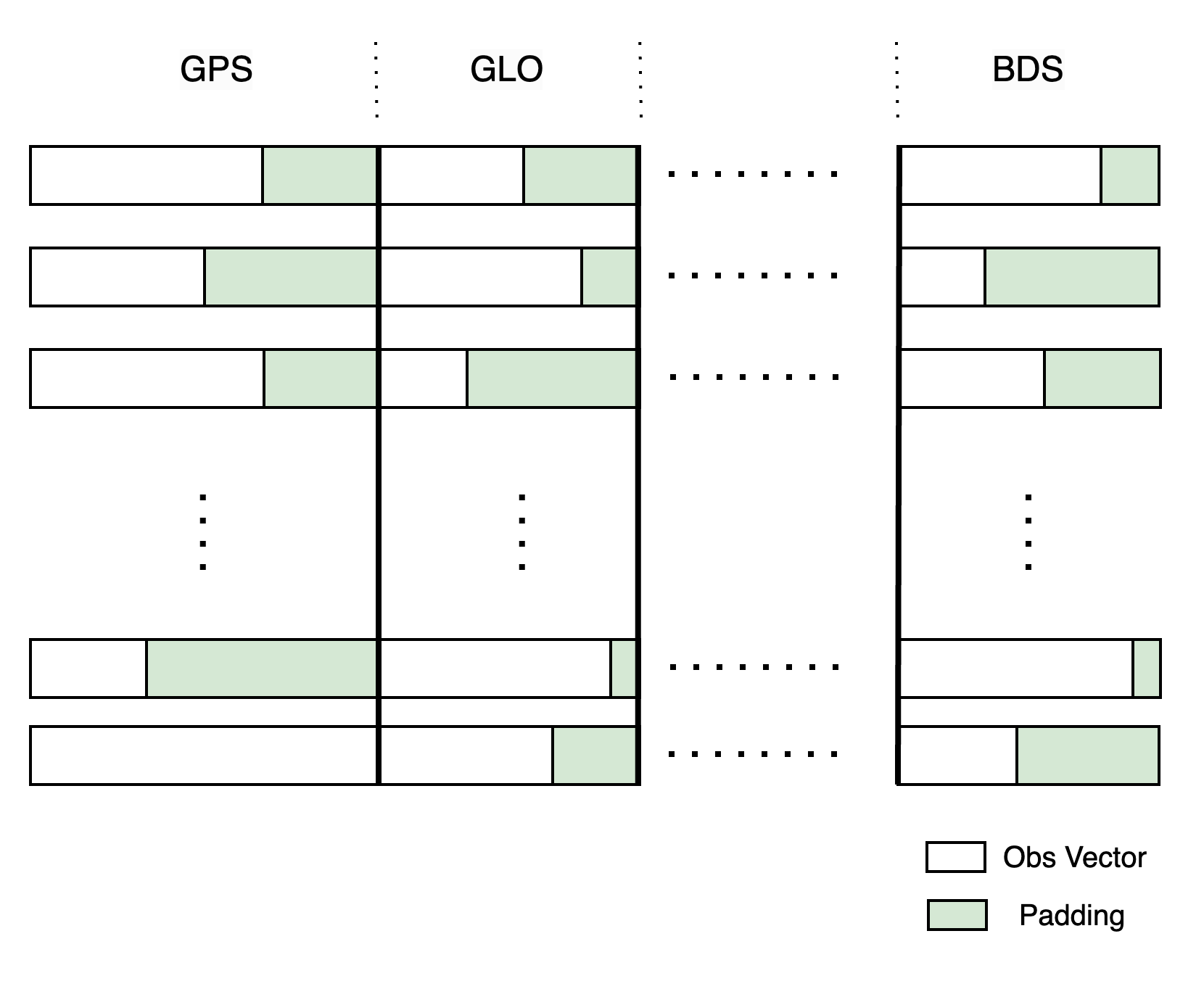
GNSS observations for each epoch arrive as a set of satellite measurements. Neural networks, however, often receive them as a sequence. We handled this by:

• sorting satellites first by constellation ID and then by elevation angle;
• padding every sorted list to the maximum satellite count.

This creates consistent input shapes and removes the need for a specialized permutation-invariant architecture.

3.3 Converting regression into classification

Directly predicting a continuous coordinate correction from raw measurements is difficult. Instead, we transform the coordinate error relative to WLS into discrete classes, using intervals between -25 m and +25 m.

Original figure unavailable — the old GitHub attachment no longer exists.

The transformation function $f(e)$ is

$$f(e) = \operatorname{sign}(e) \cdot \begin{cases} 25 & \text{if } 15 \leq |e| \leq 25 \\ 15 & \text{if } 10 \leq |e| < 15 \\ 10 & \text{if } 5 \leq |e| < 10 \\ 5 & \text{if } 2 \leq |e| < 5 \\ 2 & \text{if } 1 \leq |e| < 2 \\ 1 & \text{if } 0 < |e| < 1. \end{cases}$$

The sign preserves the direction of the error, so positive and negative corrections remain distinct.

This discretization divides the positioning error into several levels—somewhat like decomposing a signal into components. After classification, a small Mean Squared Error loss refines the final offset.

4. Model design: a BERT-like Transformer

4.1 Algebraic inspiration

WLS solves an overdetermined system by combining evidence from many equations. A Transformer attends to many inputs. In GNSS, each satellite measurement can be treated like one imperfect equation, and the model learns how those measurements relate to one another to find a better geometric fit.

4.2 BERT-like encoder

We adapt a BERT-style Transformer—commonly used for text classification, such as IMDB review analysis—to GNSS error classification:

• Input encoding: sorted and padded GNSS features are embedded into a higher-dimensional space;
• Multi-head self-attention: the model identifies which satellites and features are most reliable;
• Classification heads: discrete error classes are predicted for $\Delta x$, $\Delta y$, and $\Delta z$, then converted into a final correction offset.

4.3 Hybrid loss

The model combines classification and regression objectives:

$$\mathcal{L} = \alpha\mathcal{L}_{\text{CE}} + (1-\alpha)\mathcal{L}_{\text{MSE}},$$

where $\mathcal{L}_{\text{CE}}$ is cross-entropy for the coarse error intervals and $\mathcal{L}_{\text{MSE}}$ refines the final position. Balancing the two stabilizes training while preserving fine-grained accuracy.

5. Results

5.1 Cumulative distribution functions

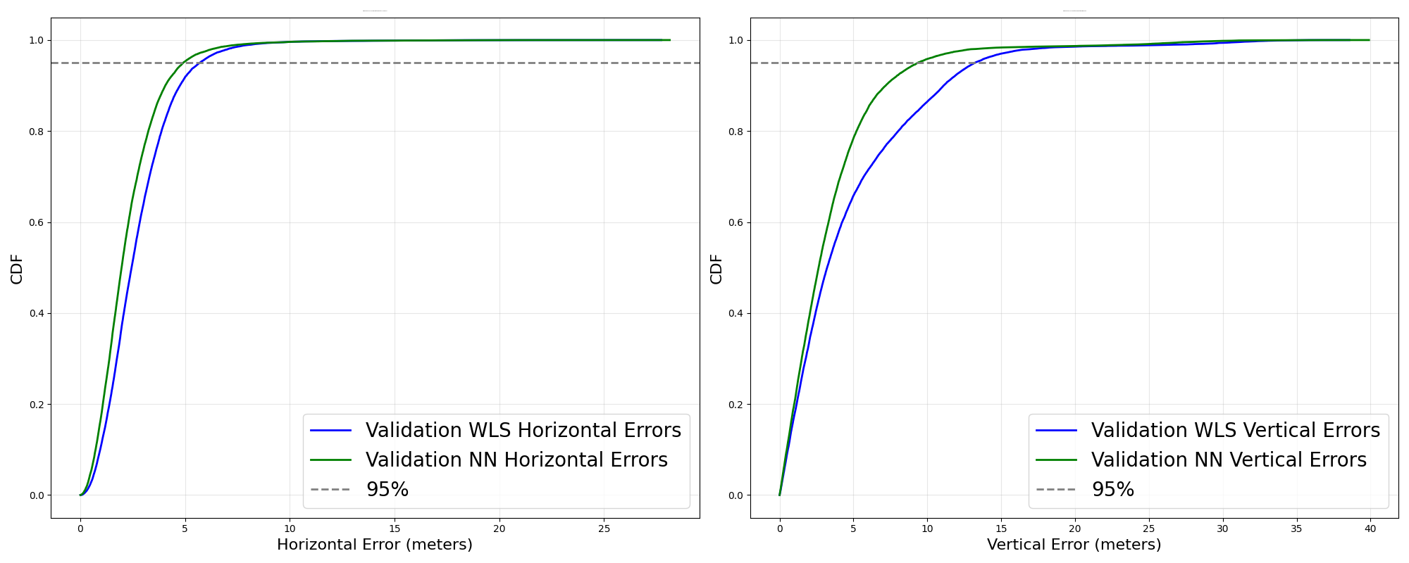
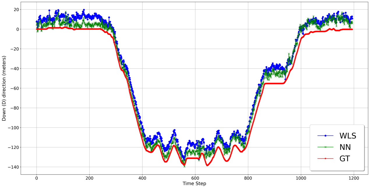
In the following figures, blue represents the WLS baseline and green represents the neural network.

5.2 Positioning-error metrics

Direction	Model	MSE	Mean	50th percentile	95th percentile
Horizontal	WLS	10.44	2.74	2.45	5.70
Horizontal	NN	7.73	2.28	1.98	4.91
Vertical	WLS	46.85	4.80	3.22	13.22
Vertical	NN	27.02	3.55	2.64	9.36

The neural network lowers every reported metric. The largest improvement appears in the vertical MSE, which falls from 46.85 to 27.02.

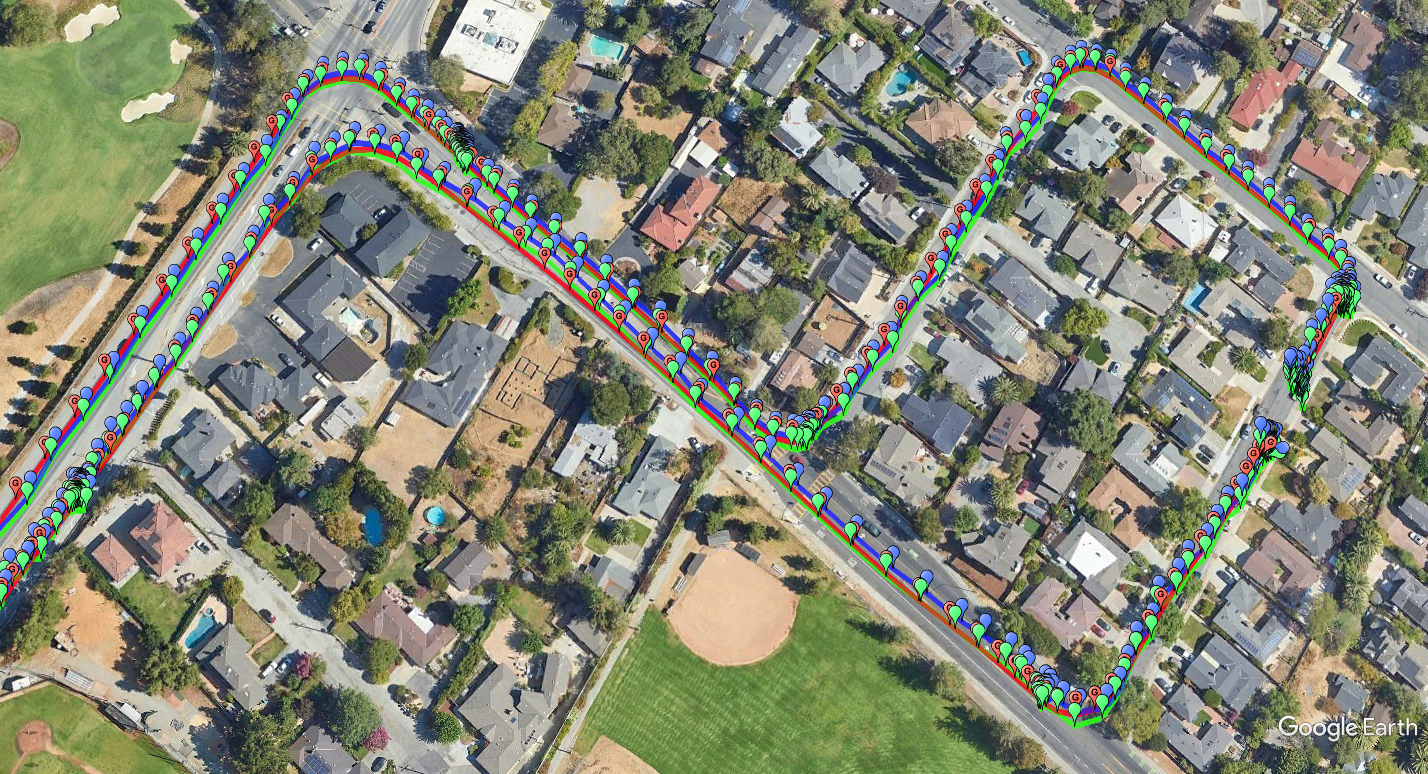
5.3 Estimated trajectories compared with ground truth

The trajectory figures use blue for WLS, green for the neural network, and red for ground truth.

Conclusion

Multipath and NLOS errors are difficult to model precisely with traditional mathematical methods. Deep learning offers a promising correction layer by learning from the environmental patterns contained in the measurements.

This system transforms a difficult-to-converge regression problem into a classification task that groups positioning errors into discrete levels. Combined with the preprocessing pipeline and hybrid loss, the approach improves positioning accuracy over the WLS baseline, particularly in challenging environments.

The result demonstrates the potential of deep learning to complement conventional GNSS positioning and provide a more robust solution for real-time smartphone positioning.

After thoughts

Although the final results show an overall improvement, some individual ideas were not validated separately because of time constraints. The loss was also aggregated and averaged across the dataset, so some traces remain less accurate than the WLS baseline. This highlights the importance of distribution differences in the data.

Future work should analyze and categorize distinct scenarios—for example, urban canyons, open fields, and mixed environments. Separating these data segments and tailoring training or evaluation to their characteristics could further improve positioning accuracy and make the model more robust across environments.